

Next: How Playpen fits the
Up: A new proposal about
Previous: Learning
In this section we illustrate the behavior of the model with a
simple simulation.![[*]](http://www.cs.indiana.edu/img/latex2html/foot_motif.gif) In this simulation a network learns both inter-MRU correlations
across different dimensions and also simple relational categories.
The simulation also illustrates how the ease of learning particular words
can depend on the match between the words and the relational
correlations that the system has already picked up on.
In this simulation a network learns both inter-MRU correlations
across different dimensions and also simple relational categories.
The simulation also illustrates how the ease of learning particular words
can depend on the match between the words and the relational
correlations that the system has already picked up on.
We first defined a set of
correlations among non-linguistic dimensions and
a set of correlations between
the non-linguistic dimensions and words.
There were two non-linguistic dimensions and four possible
micro-relations within each of these dimensions.
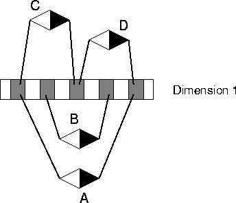
For example, micro-relation A represented a relation between a
very low value for one object and a very high value for another object
on Dimension 1, and micro-relation E represented a similar
micro-relation on Dimension 2.
The micro-relations within Dimension 1 are shown in
Figure 18.
Keep in mind that each micro-relation is a relation between values
on a particular dimension for two different objects.
Figure:
Micro-relations used in simulation. A, B, C, and D
represent possible micro-relations between features within Dimension
1. (Relations on Dimension 2, E, F, G, and H, are not shown.
They are isomorphic to the relations on Dimension 1.)
 |
Across the dimensions there were correlations between
particular micro-relations.
That is, a pair of objects with a particular relation between
their values on one dimension tended to have one or another
of a set of relations between their values on the other.
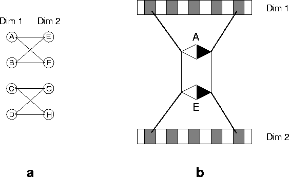
For example, micro-relation A on Dimension 1 correlated with
micro-relations E and F, but not with micro-relations G and H,
on Dimension 2.
The relational correlations are shown in
Figure 19a.
Figure 19b illustrates one of the
correlations, that between micro-relation A on Dimension 1 and
micro-relation E on Dimension 2.
Figure:
Correlations used in the simulation.
(a) The micro-relations on Dimensions 1 and 2
correlate with each other across the dimensions in
the two clusters shown.
(b) Illustration of one of the correlations.
 |
We defined two ``languages,''
an Easy language, which agrees with the non-linguistic
correlations, and a Hard language, which disagrees with the
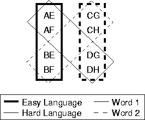
non-linguistic correlations, as shown in
Figure 20.
Each language consists of two relational words.
In the figure, the two words are indicated by the boxes with either
solid (Word 1) or dashed (Word 2) borders.
The two words in the Easy language are indicated by boxes with thick
borders (the two vertical boxes); the two words in the Hard language
are indicated by boxes with thin borders (the two diagonal boxes).
All four
words are relational; that is, they represents relations between two
separate objects.
Each word is associated with a cluster of four possible situations,
each characterized by a pairing of a micro-relation on Dimension 1 and a
micro-relation on Dimension 2.
As can be seen in
Figure 19a, each of these situations
corresponds to an actual correlation of micro-relations in the real world.
The two languages differ in terms of how these situations are grouped
for the two words.
Consider first the choice of one word over the other in the Easy
language.
In this language, Word 1 (the vertical box on the left
in Figure 20) is associated with situations
AE, AF, BE, and BF, whereas Word 2 (the vertical box on the right)
is associated with situations CG, CH, DG, and DH.
On Dimension 1, distinct sets of micro-relations are associated
with distinct words: A and B for Word 1, C and D for Word 2.
Therefore, given a pair of related objects, we can select the
appropriate word if we know their relation on Dimension 1 only;
for example, objects related by A on Dimension 1 will be referred to
with Word 1.
The same holds for Dimension 2.
E and F are associated with Word 1, G and H with Word 2.
Given a pair of objects, we can select the appropriate word if
we know their relation on Dimension 2 only.
More importantly, each of the two words in this language agrees with
the clusters of correlations in the world.
Given these correlations and the relation for a pair of objects on
Dimension 1, we know something about their relation on Dimension 2,
and both of these relations are associated with the same word.
For example, if we know that a pair of objects is associated by
relation C on Dimension 1, the correlations in the world tell us that
those objects are likely to be associated by relation G or H on
Dimension 2 (Figure Figure 19a).
But in the Easy language, both of these features of the objects (C on
Dimension 1, G or H on Dimension 2) call forth the same word, Word 1.
The same holds when we start with the Dimension 2 and predict the
value on Dimension 1.
Thus the words in the Easy language ``make sense.''
They should be relatively easy to learn because they are supported by
the correlations in the world; inferences about uncertain values on
one or the other dimension only help in the selection of the word.
Now consider the Hard language.
Word 1 in the Hard language (the solid diagonal box in
Figure 20),
is associated with four possible pairings of relations on the two
dimensions: AE, AF, DG, and DH.
For Dimension 1, the situation is as with the Easy language.
If we know that an input pair of objects has relation D on Dimension
1, we know that Word 1 is the appropriate word.
However, unlike for the Easy language, Dimension 2 is of no help in
selecting the word.
Each word can take all four possible values on Dimension 2.
In and of itself, the irrelevance of Dimension 2 for the Hard language
does not make the language difficult.
The learner could simply come to ignore that dimension and attend only
to Dimension 1.
On some accounts, this could actually make the learning task simpler.
But consider how this language relates to what goes on in the world
around the learner.
Again, because of the correlations in the world, knowing the relation
between
a pair of objects on Dimension 1 allows one to make predictions
about the relation on Dimension 2.
But, unlike for the Easy language, this prediction is of no help;
the relation on Dimension 2 is irrelevant for word selection.
Similarly, knowing the relation between two objects on Dimension 2
allows predictions to made about Dimension 1.
But for the Hard language, these predictions are of no use; the two
relations on Dimension 1 correlated with a relation on Dimension 2
(for example, C and D with G) are associated with different words.
Thus the Hard language doesn't make as much ``sense'' as the Easy language
because it fails to capitalize on the clusters of correlations
occurring in the world.
Figure:
Possible pairings of micro-relations on the two
dimensions are associated with one or the other of two words.
In the Easy language, the words agree with the non-linguistic
correlations; in the
Hard language, the words correlate only with micro-relations on Dimension
1.
 |
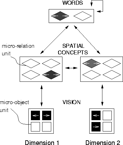
The architecture of the network used in the simulation is shown
in Figure 21.
Figure:
Network architecture. Micro-object units are represented
by squares,
micro-relation units by diamonds. Arrows indicate complete connectivity
between layers. Each MRU in the SPATIAL CONCEPTS layer
is associated with a pair of VISION
MOUs. A possible pattern across the network is shown. Darkness
indicates activation, and arrow direction indicates relative phase
angle.
 |
The goal of the experiment is to see how the different correlational
patterns both between dimensions and with the words affect the
difficulty of learning the two languages.
The network was trained and tested on two different tasks.
Training began with a Pre-Linguistic Phase in which the task was
Non-Linguistic Pattern Completion.
That is, for each trial the network was presented with a
pattern on one of the visual dimensions, representing values for two
different objects on that dimension, and expected to produce an
appropriate pattern on the other, representing the values for those
objects on that dimension.
(Note that there are always two possibilities for the appropriate
pattern.)
The network can learn to solve this task using the connections joining
the VISION and SPATIAL CONCEPTS layers or the
connections between the two SPATIAL CONCEPTS layers.
This phase continued for 30 repetitions of the relevant training
patterns (epochs).
Next, during a Linguistic Phase,
Pattern Completion training was discontinued, and the networks were
trained on Production for seven epochs.
For this task, the network was presented with a pattern on the
VISION layer, representing the values for two objects on both
dimensions, and expected to output a word.
Training in the Linguistic Phase began with weights of 0.0 connecting
the SPATIAL CONCEPTS to the WORDS units, so the network was initially
unable to produce any words.
We predicted that the Easy language would be learned faster than the
Hard language during the Production phase because the Easy language
categories agreed with the non-linguistic categories.
That is, the correlations learned during the Pre-Linguistic Phase
should support the selection of words in the Easy language but should
provide no support for the selection of words in the Hard language.
During the Pre-linguistic Phase, the networks mastered the
Pattern Completion task by learning weights between the two Hidden
layers representing the non-linguistic correlations.
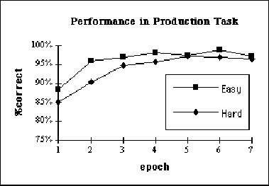
Results for the Linguistic Phase are shown in
Figure 22, starting with performance after one
epoch.
Figure:
Results for simulation. The Easy language is
learned faster than the Hard language.
 |
The data were submitted to a 2(Language)  7(Epoch) analysis of
variance for a mixed design. This analysis revealed a main effect of
epoch, indicating that the networks get better as they receive more
training. More importantly, as predicted, there is a main effect of
language (p<.001). Thus, as predicted,
the Easy language is learned faster than
the Hard language, although by the end of the training the two
networks have comparable performance. No interactions between language
and epoch were found.


Next: How Playpen fits the
Up: A new proposal about
Previous: Learning
Michael Gasser
1999-09-08
![[*]](http://www.cs.indiana.edu/img/latex2html/foot_motif.gif) In this simulation a network learns both inter-MRU correlations
across different dimensions and also simple relational categories.
The simulation also illustrates how the ease of learning particular words
can depend on the match between the words and the relational
correlations that the system has already picked up on.
In this simulation a network learns both inter-MRU correlations
across different dimensions and also simple relational categories.
The simulation also illustrates how the ease of learning particular words
can depend on the match between the words and the relational
correlations that the system has already picked up on.
