Digital Signal Processing Overview

Digital Signal Processing Overview

R. Port, October 3, 2007

I. Digital Representation of a Waveform

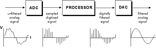
A digital signal processing system takes a continuous sound wave as input, feeds it through an analog low-pass filter (an anti-aliassing filter) to remove all frequencies above half the sampling rate (see Nyquist's sampling theorem). This Analog-to-Digital Converter (ADC) filters and samples the wave amplitude at equally-spaced time intervals and generates a simple list of ordered sample values in successive memory locations in the computer. The sample values, representing amplitudes, are encoded using some number of bits that determines how accurately the samples are measured. The Processor is a computer that applies numerical operations to the sampled waves. In the figure below, it appears the processor has low-pass filtered the signal, thus removing the jumpy irregularities in the input wave. When the signal is converted back into an audio signal by the Digital-Analog Converter (DAC), there will be jagged irregularities (shown below on this page) that are quanization errors. Of course, these will lie above the Nyquist frequency, so the new analog signal (back in realtime) needs another analog, low-pass filter on output since everything above the Nyquist frequency is a noisy artefact.

A. Sampling theorem: `Nyquist freq' = (sampling rate)/2

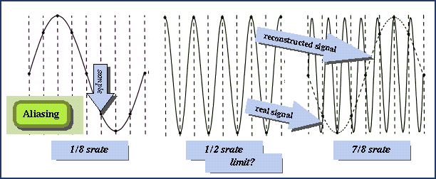
Aliassing problem (frequencies above Nyquist frequency get mapped to lower frequencies). The leftmost wave below has 8 samples per cycle (that is, the frequency is 1/8 the sample rate (the srate). The middle curve is the highest frequency that can be represented by this sample rate. The rightmost figure is much too fast, so the sampled wave will sound like (be aliassed as) the slow dotted curve (which is identical to the leftmost curve).

The image “http://ccrma.stanford.edu/CCRMA/Courses/220a:1996/Lectures/2/Images/_03a_Aliasing.gif” cannot be displayed, because it contains errors.

Solution: apply an input filter before sampling to remove all unwanted inputs. Any energy remaining above the Nyquist frequency will be mapped onto lower frequencies. Of course, on modern digital equipment, this filtering is taken care of for you.
for CD standard, sampling rate = 44.1 kHz, so the Nyquist freq = 22.05 kHz. (Human hearing ends at 20 kHz.)

B. Quantization of amplitude (limited set of amplitude values). When the sampled signal is converted back into realtime, of course, there are only assigned values specified at the sample points. The output signal will just be flat until the next sample comes along. These flat spots will be perceived by a listener as a high-frequency signal (above the Nyquist freq), but it will be noise . So the red curve below must be smoothed (lowpass filtered) into the green curve below in order to sound right. Of course, if the sample rate is that of the commercial CD standard, then this noise will be above the limits of human hearing -- so your own ear can serve as the lowpass quantization filter. Indeed, since loudspeakers do not normally produce sounds above 20 kHzm, they too can also serve as this lowpass output filter.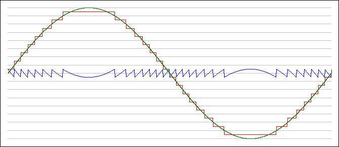

Quantization noise - the difference between the original and the quantized signal. The difference between the green signal curve and the red output curve is copied below in blue.

Output filters are needed (to smooth away quantization noise)

For the commercial CD audio standard (sestablished in 1980), quantization is 16 bits = 2^16 = 65,536 amplitude values

Thus, 1 second of audio at CD quality requires 16 bits X 44.1k = 705,600 bits. Of course, for speech research, one normally needs only about 5 kHz bandwidth (for a sampling rate of 10kHz) - about half of the CD standard.

II. Digital Filtering - numerical methods for filtering sampled signals. Sample values at each point in time are identified with the integers, n. The sampled amplitudes are identified here as X_n and a_ns will be the coefficients for modifying each amplitude. The image “http://cara.gsu.edu/courses/MI_3110/filters1/fltimg3.jpg” cannot be displayed, because it contains errors.

The image “http://cara.gsu.edu/courses/MI_3110/filters1/fltimg3.jpg” cannot be displayed, because it contains errors.

A. Primitive low-pass digital filter - For example, a running average of 2 (or more) adjacent samples. Thus, take sample X_n and sample X_n+1, add their amplitudes, and divide by 2. This is equivalent to taking half the amplitude of sample X_n and adding half of X_n+1. (The mathematical term for such a `running average-like' calculation is convolution: apply the operation, move over one time step, apply it again. Repeat until you run out of samples.) The number of coefficients used is the order of the filter, so the `running average of 2 adjacent samples' has order 2.

more generally, for a primitive smoothing (or low-pass) filter,

Y₀ = a_-2X_-2 + a_-1X_-1 + a₀X₀ +...a_mX_m, where

(1) X₀ is an input sample value, X_-1is the previous sample value and Y₀is an output sample value (interpret the digits and m as subscript indices)
(2) the a's are filter coefficients that are multiplied times the sample amplitudes, X, and the coefficients, a generally sum to 1 (although sometimes the coefficients can be negative. Of course, if they sum to something greater than 1, then the filter is also an amplifier) and
(3) m (number of coefficients) is called the `order' of the filter.

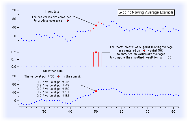
Here is a digital signal processed by a 5th-order moving-average filter. It averages 5 adjacent samples by multiplying each by .2, then summing. You can see how the signal is smoothed in the bottom display. The higher-frequency components of the function have been removed. The equation for this filter is: Y ₀ = .2X _-2 + .2X _-1 + .2X₀ + .2X₊₁ + .2X₊₂ It is illustrate below as the 5 red lines in the middle panel.

The image “http://www.wavemetrics.com/Products/igorpro/dataanalysis/signalprocessing/smoothingpix/movingaveragedemo.png” cannot be displayed, because it contains errors.

Impulse response: response of the filter to a single sample of 1 embedded among adjacent samples of 0 -- roughly equivalent to tapping a bell or pinging the resonator. Below the red impulse of 1 causes the filter to respond with a fading oscillation.

B. Primitive high-pass filter

`first-difference filter' - Subtract adjacent samples to flatten out a lower-frequency trend in the sampled data. Rapid changes between adjacent samples are preserved, but the value that both samples share is dropped away. So an input sequence like [2,6,3,7,4,8,5,9] comes out of the filter as [+4,-3,+4,-3,+4,-3,+4].

Y₀ = a₀X₀ - a₁X₁

for various filters, the coefficients may be positive or negative. Notice that it matters very little if we use X_-1 and X₀or X₊₁and X₀-- it just shifts the data points one sample point to the left or right.

C. General properties

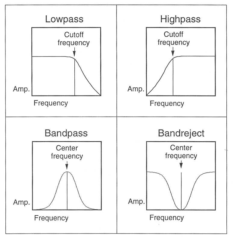
A digital filter can be made to exhibit any spectral shape you want. And mathematical methods for finding the correct form of the equation exist.
Generally, to make a filter with more peaks (or `poles' as they are sometimes called) or for sharper cutoffs and smaller ripples, more coefficients are required.

III. Fast Fourier Transform, a method for doing general Fourier analysis on sampled signals efficiently. In order for the method to be applied, one must specify the number of sample points employed (that is, the time window for the spectrum) as a power of 2 (that is, as either 4, 8, 16,...256, 1024,..., etc). Sampling, eg, at 16k Hz means 1 ms = 80 samples, so a 256 point FFT looks at 3.2 ms and a 512 point FFT looks at 6.4 ms. At the CD standard, 512 sample points is about 1 ms.

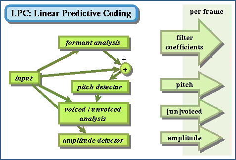
IV. Linear Predictive Coding (LPC). A method of speech coding that constructs a digital filter that will model a short segment (called a frame) of a speech waveform using many fewer bits than the explicit waveform itself requires. The coefficients and other parameters are then used to resynthesize the original speech. LPC image

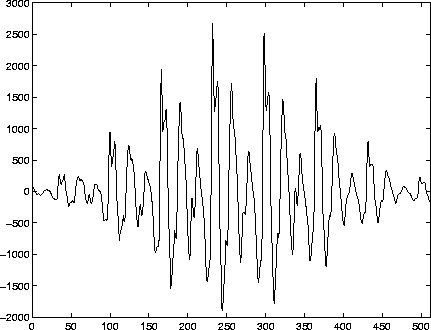
First, it turns out that simply chopping a frame from a speech signal creates artifacts dependent on the duration of the frame. To avoid these artifacts, the frame needs to be feathered at both ends, that is the amplitude of the waveform needs to be gradually reduced toward zero at each end. Two popular functions are the `Hamming window' and the `Hanning window'. The wave is multiplied by the window (with values between 0 and 1) to create a wave like that below.

The image “http://svr-www.eng.cam.ac.uk/~ajr/SA95/img75.gif” cannot be displayed, because it contains errors.

Then LPC determines the portions of the speech frame (often about 20 ms long) that are voiced from the voiceless parts. For the voiced portions, it measures the F0 (based on the distance between apparent pulses). It also measures the mean amplitude of the frame.
The LPC algorithm computes a set of filter coefficients (where the LPC order is the number of computed coefficients - usually between 6 and 20) that will reconstruct a model of the wave stretch within the frame.
This set of coefficients can then be used to approximately reconstruct (ie, synthesize) many sample points from a small number of coefficients plus indication of whether to excite the filter with noise or pitch pulses, and the location of pitch pulses in time (eg, the F0). Thus, a frame containing 2 pitch periods (about 20 ms), during which the vocal tract shape does not change very much, would contain (if sampled at 10kHz) 200 samples. A set of only 12-16 LPC coefficients plus 2 impulses (one for each pitch period) can generate the whole frame of 200 samples well enough to yield quite natural sounding speech.
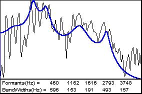
The picture above shows an FFT of a vowel frame (an [a]) and the computed LPC spectrum (which appears to employ 12 coefficients).
Rule of Thumb 1: Two (2) coefficients are needed for each spectral peak that one wishes to model, including a `peak' at frequency 0 to model the overall downward slope of the spectrum. Thus 12 coefficients will model about 5 formants in the frame plus the spectral slope.
Rule of Thumb 2: As the frames get longer (to economize on bits) the sensitivity (of the LPC representation) to change in the signal gets weaker. (Since the method averages the spectrum over the frame.) But as the frames get shorter, you will use more coefficients per second, so the economy of encoding is reduced.
Notice that the LPC algorithm calculates the spectrum without differentiating the source spectrum from the filter spectrum, the LPC coefficients model the product of both. This is because LPC uses only a unit pulse (a single sample with the value of 1) to simulate a glottal pulse (which looks quite different than an impulse that is one sample wide).
Some uses of LPC in the phonetics lab include (1) since the pitch pulses are extracted from the signal before the LPC encoding, it is a useful lab tool for manipulating F0 artificially. You just replace the file of pulses with a different file. (2) The LPC spectrum offers a description of the speech spectrum that is easier to interpret than the FFT. Indeed, programs that extract the formants of speech usually do LPC first and compute the LPC spectrum, then seek the peaks that are formants. (Wavesurfer does it this way.)